
- Optical Transceivers
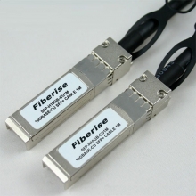
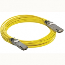
- SFP+ Transceivers
- XENPAK Transceivers
- XFP Transceivers
- X2 Transceivers
- SFP Transceivers
- Compatible SFP
- 3Com SFP
- Alcatel-Lucent SFP
- Allied Telesis SFP
- Avaya SFP
- Brocade SFP
- Cisco SFP
- D-Link SFP
- Dell SFP
- Enterasys SFP
- Extreme SFP
- Force10 SFP
- Foundry SFP
- H3C SFP
- HP SFP
- Huawei SFP
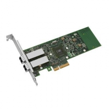
- Intel SFP
- Juniper SFP
- Linksys SFP
- Marconi SFP
- McAfee SFP
- Netgear SFP
- Nortel SFP
- Planet SFP
- Q-logic SFP
- Redback SFP
- SMC SFP
- SUN SFP
- TRENDnet SFP
- ZYXEL SFP
- Other SFP
- FE SFP
- GE SFP
- OC3 SFP
- OC12 SFP
- OC48 SFP
- Copper SFP
- CWDM SFP
- DWDM SFP
- BIDI SFP
- Fiber Channel SFP
- Multi-Rate SFP
- SGMII SFP
- Compatible SFP
- GBIC Transceivers
- Passive Components
- Networking
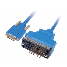
- Cables
- Equipments
- Tools
- Special Offers
Brands

Industry News

Fiber Optic Wiki

Attenuation Dead Zone
Dead zone is classified in two ways. Firstly, an "Event Dead Zone" is related to a reflective discrete optical event. In this situation, the measured dead zone will depend on a combination of the pulse length, and the size of the reflection. Secondly, an "Attenuation Dead Zone" is related to a non-reflective event.
A long signal integration time effectively increases OTDR sensitivity by averaging the receiver output. The sensitivity increases with the square root of the integration time. So if the integration time is increased by 16 times, the sensitivity increases by a factor of 4. This imposes a sensitivity practical limit, with integration times of seconds to a few minutes.
The dynamic range of an OTDR is usually specified as the attenuation level where the measured signal gets lost in the detection noise level, for a particular combination of pulse length and signal integration time. This number is easy to deduce by inspection of the output trace, and is useful for comparison, but is not very useful in practice, since at this point the measured values are random. So the practical measuring range is smaller, depending on required attenuation measurement resolution.
When an OTDR is used to measure the attenuation of multiple joined fiber lengths, the output trace can incorrectly show a joint as having gain, instead of loss. The reason for this is that adjacent fibers may have different backscatter coefficients, so the second fiber reflects more light than the first fiber, with the same amount of light travelling through it. If the OTDR is placed at the other end of this same fiber pair, it will measure an abnormally high loss at that joint. However if the two signals are then combined, the correct loss will be obtained. For this reason, it is common OTDR practice to measure and combine the loss from both ends of a link, so that the loss of cable joints, and end to end loss, can be more accurately measured.
The theoretical distance measuring accuracy of an OTDR is extremely good, since it is based on software and a crystal clock with an inherent accuracy of better than 0.01%. This aspect does not need subsequent calibration since practical cable length measuring accuracy is typically limited to about 1% due to: The cable length is not the same as the fiber length, the speed of light in the fiber is known with limited accuracy (the refractive index is only specified to 3 significant figures such as e.g. 1.45 etc.), and cable length markers have limited accuracy (0.5% – 1%).
An OTDR excels at identifying the existence of unacceptable point loss or return loss in cables. Its ability to accurately measure absolute end-to-end cable loss or return loss can be quite poor, so cable acceptance usually includes an end-to-end test with a light source and power meter, and optical return loss meter. Its ability to exactly locate a hidden cable fault is also limited, so for fault-finding it may be augmented with other localised tools such as a red laser fault locator, clip-on identifier, or "Cold Clamp" optical cable marker.
July 22, 2011
Featured


Bestsellers


Registered Names and Trademarks are the copyright and property of their respective owners.
Copyright © 2025 Fiberise(A company of Cablexa Ltd). All rights reserved.
Copyright © 2025 Fiberise(A company of Cablexa Ltd). All rights reserved.